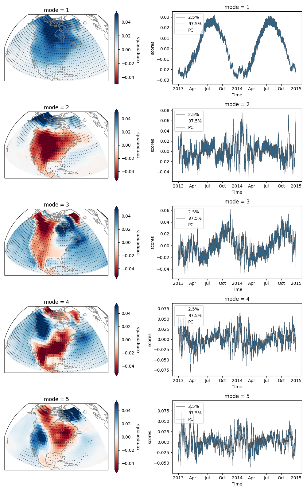
Significance testing of EOF analysis via bootstrap

Test the significance of individual modes and obtain confidence intervals for both EOFs and PCs.

# Load packages and data:
import numpy as np
import xarray as xr
import matplotlib.pyplot as plt
from matplotlib.gridspec import GridSpec
from cartopy.crs import Orthographic, PlateCarree

from xeofs.models import EOF
from xeofs.validation import EOFBootstrapper

t2m = xr.tutorial.load_dataset("air_temperature")["air"]

Perform EOF analysis

model = EOF(n_modes=5, standardize=False)
model.fit(t2m, dim="time")
expvar = model.explained_variance_ratio()
components = model.components()
scores = model.scores()

Perform bootstrapping of the model to identy the number of significant modes. We perform 50 bootstraps. Note - if computationallly feasible - you typically want to choose higher numbers of bootstraps e.g. 1000.

n_boot = 50

bs = EOFBootstrapper(n_bootstraps=n_boot)
bs.fit(model)
bs_expvar = bs.explained_variance()
ci_expvar = bs_expvar.quantile([0.025, 0.975], "n")  # 95% confidence intervals

q025 = ci_expvar.sel(quantile=0.025)
q975 = ci_expvar.sel(quantile=0.975)

is_significant = q025 - q975.shift({"mode": -1}) > 0
n_significant_modes = (
    is_significant.where(is_significant is True).cumsum(skipna=False).max().fillna(0)
)
print("{:} modes are significant at alpha=0.05".format(n_significant_modes.values))

  0%|          | 0/50 [00:00<?, ?it/s]
  2%|▏         | 1/50 [00:00<00:13,  3.65it/s]
  4%|▍         | 2/50 [00:00<00:12,  3.85it/s]
  6%|▌         | 3/50 [00:00<00:12,  3.89it/s]
  8%|▊         | 4/50 [00:01<00:11,  3.93it/s]
 10%|█         | 5/50 [00:01<00:11,  3.93it/s]
 12%|█▏        | 6/50 [00:01<00:11,  3.75it/s]
 14%|█▍        | 7/50 [00:01<00:11,  3.82it/s]
 16%|█▌        | 8/50 [00:02<00:10,  3.85it/s]
 18%|█▊        | 9/50 [00:02<00:10,  3.89it/s]
 20%|██        | 10/50 [00:02<00:10,  3.91it/s]
 22%|██▏       | 11/50 [00:02<00:10,  3.84it/s]
 24%|██▍       | 12/50 [00:03<00:09,  3.86it/s]
 26%|██▌       | 13/50 [00:03<00:09,  3.89it/s]
 28%|██▊       | 14/50 [00:03<00:09,  3.93it/s]
 30%|███       | 15/50 [00:03<00:08,  3.92it/s]
 32%|███▏      | 16/50 [00:04<00:08,  3.89it/s]
 34%|███▍      | 17/50 [00:04<00:08,  3.91it/s]
 36%|███▌      | 18/50 [00:04<00:08,  3.93it/s]
 38%|███▊      | 19/50 [00:04<00:07,  3.94it/s]
 40%|████      | 20/50 [00:05<00:07,  3.96it/s]
 42%|████▏     | 21/50 [00:05<00:07,  3.96it/s]
 44%|████▍     | 22/50 [00:05<00:07,  3.97it/s]
 46%|████▌     | 23/50 [00:05<00:06,  3.95it/s]
 48%|████▊     | 24/50 [00:06<00:06,  3.95it/s]
 50%|█████     | 25/50 [00:06<00:06,  3.95it/s]
 52%|█████▏    | 26/50 [00:06<00:06,  3.96it/s]
 54%|█████▍    | 27/50 [00:06<00:05,  3.96it/s]
 56%|█████▌    | 28/50 [00:07<00:05,  3.97it/s]
 58%|█████▊    | 29/50 [00:07<00:05,  3.97it/s]
 60%|██████    | 30/50 [00:07<00:05,  3.98it/s]
 62%|██████▏   | 31/50 [00:07<00:04,  3.97it/s]
 64%|██████▍   | 32/50 [00:08<00:04,  3.84it/s]
 66%|██████▌   | 33/50 [00:08<00:04,  3.86it/s]
 68%|██████▊   | 34/50 [00:08<00:04,  3.90it/s]
 70%|███████   | 35/50 [00:08<00:03,  3.91it/s]
 72%|███████▏  | 36/50 [00:09<00:03,  3.92it/s]
 74%|███████▍  | 37/50 [00:09<00:03,  3.93it/s]
 76%|███████▌  | 38/50 [00:09<00:03,  3.94it/s]
 78%|███████▊  | 39/50 [00:09<00:02,  3.94it/s]
 80%|████████  | 40/50 [00:10<00:02,  3.93it/s]
 82%|████████▏ | 41/50 [00:10<00:02,  3.88it/s]
 84%|████████▍ | 42/50 [00:10<00:02,  3.88it/s]
 86%|████████▌ | 43/50 [00:11<00:01,  3.73it/s]
 88%|████████▊ | 44/50 [00:11<00:01,  3.79it/s]
 90%|█████████ | 45/50 [00:11<00:01,  3.76it/s]
 92%|█████████▏| 46/50 [00:11<00:01,  3.74it/s]
 94%|█████████▍| 47/50 [00:12<00:00,  3.78it/s]
 96%|█████████▌| 48/50 [00:12<00:00,  3.61it/s]
 98%|█████████▊| 49/50 [00:12<00:00,  3.50it/s]
100%|██████████| 50/50 [00:12<00:00,  3.51it/s]
100%|██████████| 50/50 [00:12<00:00,  3.85it/s]
0.0 modes are significant at alpha=0.05

The bootstrapping procedure identifies 3 significant modes. We can also compute the 95 % confidence intervals of the EOFs/PCs and mask out insignificant elements of the obtained EOFs.

ci_components = bs.components().quantile([0.025, 0.975], "n")
ci_scores = bs.scores().quantile([0.025, 0.975], "n")

is_sig_comps = np.sign(ci_components).prod("quantile") > 0

Summarize the results in a figure.

lons, lats = np.meshgrid(is_sig_comps.lon.values, is_sig_comps.lat.values)
proj = Orthographic(central_latitude=30, central_longitude=-80)
kwargs = {"cmap": "RdBu", "vmin": -0.05, "vmax": 0.05, "transform": PlateCarree()}

fig = plt.figure(figsize=(10, 16))
gs = GridSpec(5, 2)
ax1 = [fig.add_subplot(gs[i, 0], projection=proj) for i in range(5)]
ax2 = [fig.add_subplot(gs[i, 1]) for i in range(5)]

for i, (a1, a2) in enumerate(zip(ax1, ax2)):
    a1.coastlines(color=".5")
    components.isel(mode=i).plot(ax=a1, **kwargs)
    a1.scatter(
        lons,
        lats,
        is_sig_comps.isel(mode=i).values * 0.5,
        color="k",
        alpha=0.5,
        transform=PlateCarree(),
    )
    ci_scores.isel(mode=i, quantile=0).plot(ax=a2, color=".3", lw=".5", label="2.5%")
    ci_scores.isel(mode=i, quantile=1).plot(ax=a2, color=".3", lw=".5", label="97.5%")
    scores.isel(mode=i).plot(ax=a2, lw=".5", alpha=0.5, label="PC")
    a2.legend(loc=2)

plt.tight_layout()
plt.savefig("bootstrap.jpg")