Rotated Maximum Covariance Analysis

Rotated Maximum Covariance Analysis (MCA) between two data sets.

# Load packages and data:
import numpy as np
import xarray as xr
import matplotlib.pyplot as plt
from matplotlib.gridspec import GridSpec
from cartopy.crs import Orthographic, PlateCarree
from cartopy.feature import LAND

from xeofs.models import MCA, MCARotator

Create 2 different DataArrays

t2m = xr.tutorial.load_dataset("air_temperature")["air"]
da1 = t2m.isel(lon=slice(0, 26))
da2 = t2m.isel(lon=slice(27, None))

Perform MCA

mca = MCA(n_modes=20, standardize=False, use_coslat=True)
mca.fit(da1, da2, dim="time")

<xeofs.models.mca.MCA object at 0x7fa6f9945b10>

Apply Varimax-rotation to MCA solution

rot = MCARotator(n_modes=10)
rot.fit(mca)

<xeofs.models.mca_rotator.MCARotator object at 0x7fa6f935a610>

Get rotated singular vectors, projections (PCs), homogeneous and heterogeneous patterns:

singular_vectors = rot.components()
scores = rot.scores()
hom_pats, pvals_hom = rot.homogeneous_patterns()
het_pats, pvals_het = rot.heterogeneous_patterns()

When two fields are expected, the output of the above methods is a list of length 2, with the first and second entry containing the relevant object for X and Y. For example, the p-values obtained from the two-sided t-test for the homogeneous patterns of X are:

pvals_hom[0]

<xarray.DataArray 'pvalues_of_left_homogeneous_patterns' (mode: 10, lat: 25,
                                                          lon: 26)> Size: 52kB
5.921e-81 4.092e-64 6.235e-58 5.975e-49 ... 0.001974 0.005479 0.01494 0.03604
Coordinates:
  * lat      (lat) float32 100B 15.0 17.5 20.0 22.5 25.0 ... 67.5 70.0 72.5 75.0
  * lon      (lon) float32 104B 200.0 202.5 205.0 207.5 ... 257.5 260.0 262.5
  * mode     (mode) int64 80B 1 2 3 4 5 6 7 8 9 10
Attributes:
    model:             Rotated MCA
    n_modes:           10
    power:             1
    max_iter:          1000
    rtol:              1e-08
    squared_loadings:  False
    compute:           True
    software:          xeofs
    version:           2.3.2
    date:              2024-03-31 21:13:29

xarray.DataArray

'pvalues_of_left_homogeneous_patterns'

• mode: 10
• lat: 25
• lon: 26

• 5.921e-81 4.092e-64 6.235e-58 5.975e-49 ... 0.005479 0.01494 0.03604

  array([[[5.92059789e-081, 4.09191468e-064, 6.23501668e-058, ...,
           4.45360714e-046, 7.99438654e-107, 6.96004798e-234],
          [9.61447004e-109, 4.31051559e-079, 2.41959746e-054, ...,
           1.13321801e-079, 1.17049272e-086, 1.58781875e-105],
          [3.66002675e-169, 1.03632537e-150, 5.85996512e-088, ...,
           2.66120502e-037, 1.39447628e-071, 1.89940824e-183],
          ...,
          [0.00000000e+000, 0.00000000e+000, 0.00000000e+000, ...,
           0.00000000e+000, 0.00000000e+000, 0.00000000e+000],
          [0.00000000e+000, 0.00000000e+000, 0.00000000e+000, ...,
           0.00000000e+000, 0.00000000e+000, 0.00000000e+000],
          [0.00000000e+000, 0.00000000e+000, 0.00000000e+000, ...,
           0.00000000e+000, 0.00000000e+000, 0.00000000e+000]],
  
         [[0.00000000e+000, 0.00000000e+000, 0.00000000e+000, ...,
           2.14893389e-115, 1.25702836e-037, 3.79415536e-010],
          [0.00000000e+000, 0.00000000e+000, 0.00000000e+000, ...,
           3.68453572e-006, 4.54439381e-001, 7.47363320e-001],
          [5.82895742e-304, 1.04472081e-286, 1.67982320e-322, ...,
           3.12432619e-031, 2.97912134e-009, 3.83994158e-013],
  ...
          [3.81949570e-033, 1.24768007e-035, 9.83759619e-037, ...,
           1.08209176e-007, 2.09241996e-007, 9.75023943e-007],
          [7.63519595e-018, 1.85000852e-018, 1.85005574e-018, ...,
           1.47665876e-002, 2.23167561e-002, 3.74987366e-002],
          [5.23836620e-013, 5.59341926e-014, 1.46543909e-014, ...,
           7.79688373e-001, 7.97073112e-001, 8.38056703e-001]],
  
         [[1.33002815e-001, 3.88098908e-002, 2.39380431e-003, ...,
           9.33550484e-001, 6.41356878e-001, 5.12875506e-001],
          [2.47968728e-002, 1.49402627e-002, 1.01798500e-003, ...,
           9.48619892e-001, 3.16362047e-001, 6.29374288e-002],
          [1.00284835e-002, 8.50789082e-002, 1.51714932e-001, ...,
           2.62220485e-001, 1.27839757e-002, 1.43415444e-004],
          ...,
          [6.95257678e-010, 1.10866744e-010, 2.79779292e-011, ...,
           2.20336993e-004, 2.58482090e-003, 2.44606634e-002],
          [2.08884879e-002, 1.93782160e-002, 2.08180373e-002, ...,
           3.74567689e-004, 2.56338312e-003, 1.63483626e-002],
          [9.06097806e-001, 8.65003190e-001, 8.39191905e-001, ...,
           5.47880876e-003, 1.49440220e-002, 3.60354439e-002]]])

• Coordinates: (3)
  • lat
    (lat)
    float32
    15.0 17.5 20.0 ... 70.0 72.5 75.0

    array([15. , 17.5, 20. , 22.5, 25. , 27.5, 30. , 32.5, 35. , 37.5, 40. , 42.5,
           45. , 47.5, 50. , 52.5, 55. , 57.5, 60. , 62.5, 65. , 67.5, 70. , 72.5,
           75. ], dtype=float32)

  • lon
    (lon)
    float32
    200.0 202.5 205.0 ... 260.0 262.5

    array([200. , 202.5, 205. , 207.5, 210. , 212.5, 215. , 217.5, 220. , 222.5,
           225. , 227.5, 230. , 232.5, 235. , 237.5, 240. , 242.5, 245. , 247.5,
           250. , 252.5, 255. , 257.5, 260. , 262.5], dtype=float32)

  • mode
    (mode)
    int64
    1 2 3 4 5 6 7 8 9 10

    array([ 1,  2,  3,  4,  5,  6,  7,  8,  9, 10])

• Indexes: (3)
  • mode
    PandasIndex

    PandasIndex(Index([1, 2, 3, 4, 5, 6, 7, 8, 9, 10], dtype='int64', name='mode'))

  • lat
    PandasIndex

    PandasIndex(Index([15.0, 17.5, 20.0, 22.5, 25.0, 27.5, 30.0, 32.5, 35.0, 37.5, 40.0, 42.5,
           45.0, 47.5, 50.0, 52.5, 55.0, 57.5, 60.0, 62.5, 65.0, 67.5, 70.0, 72.5,
           75.0],
          dtype='float32', name='lat'))

  • lon
    PandasIndex

    PandasIndex(Index([200.0, 202.5, 205.0, 207.5, 210.0, 212.5, 215.0, 217.5, 220.0, 222.5,
           225.0, 227.5, 230.0, 232.5, 235.0, 237.5, 240.0, 242.5, 245.0, 247.5,
           250.0, 252.5, 255.0, 257.5, 260.0, 262.5],
          dtype='float32', name='lon'))

• Attributes: (10)

  model :

  Rotated MCA

  n_modes :

  10

  power :

  1

  max_iter :

  1000

  rtol :

  1e-08

  squared_loadings :

  False

  compute :

  True

  software :

  xeofs

  version :

  2.3.2

  date :

  2024-03-31 21:13:29

Create a mask to identifiy where p-values are below 0.05

hom_mask = [values < 0.05 for values in pvals_hom]
het_mask = [values < 0.05 for values in pvals_het]

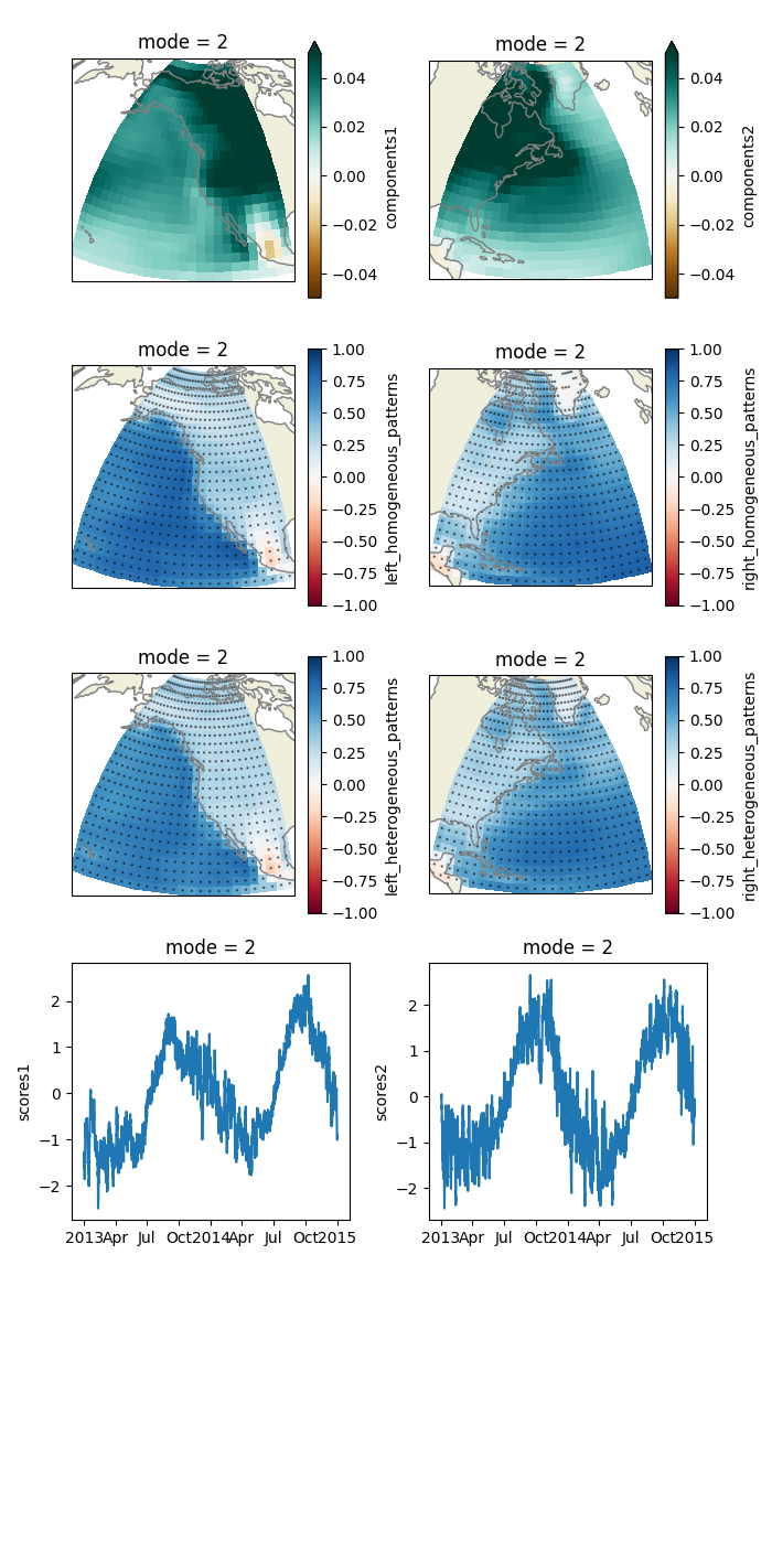
Plot some relevant quantities of mode 2.

lonlats = [
    np.meshgrid(pvals_hom[0].lon.values, pvals_hom[0].lat.values),
    np.meshgrid(pvals_hom[1].lon.values, pvals_hom[1].lat.values),
]
proj = [
    Orthographic(central_latitude=30, central_longitude=-120),
    Orthographic(central_latitude=30, central_longitude=-60),
]
kwargs1 = {"cmap": "BrBG", "vmin": -0.05, "vmax": 0.05, "transform": PlateCarree()}
kwargs2 = {"cmap": "RdBu", "vmin": -1, "vmax": 1, "transform": PlateCarree()}

mode = 2

fig = plt.figure(figsize=(7, 14))
gs = GridSpec(5, 2)
ax1 = [fig.add_subplot(gs[0, i], projection=proj[i]) for i in range(2)]
ax2 = [fig.add_subplot(gs[1, i], projection=proj[i]) for i in range(2)]
ax3 = [fig.add_subplot(gs[2, i], projection=proj[i]) for i in range(2)]
ax4 = [fig.add_subplot(gs[3, i]) for i in range(2)]

for i, a in enumerate(ax1):
    singular_vectors[i].sel(mode=mode).plot(ax=a, **kwargs1)

for i, a in enumerate(ax2):
    hom_pats[i].sel(mode=mode).plot(ax=a, **kwargs2)
    a.scatter(
        lonlats[i][0],
        lonlats[i][1],
        hom_mask[i].sel(mode=mode).values * 0.5,
        color="k",
        alpha=0.5,
        transform=PlateCarree(),
    )
for i, a in enumerate(ax3):
    het_pats[i].sel(mode=mode).plot(ax=a, **kwargs2)
    a.scatter(
        lonlats[i][0],
        lonlats[i][1],
        het_mask[i].sel(mode=mode).values * 0.5,
        color="k",
        alpha=0.5,
        transform=PlateCarree(),
    )

for i, a in enumerate(ax4):
    scores[i].sel(mode=mode).plot(ax=a)
    a.set_xlabel("")


for a in np.ravel([ax1, ax2, ax3]):
    a.coastlines(color=".5")
    a.add_feature(LAND)

plt.tight_layout()
plt.savefig("rotated_mca.jpg")