Note
Go to the end to download the full example code
Removing nonlinear trends with EEOF analysis#
This tutorial illustrates the application of Extended EOF (EEOF) analysis to isolate and remove nonlinear trends within a dataset.
Let’s begin by setting up the required packages and fetching the data.
import xarray as xr
import xeofs as xe
import matplotlib.pyplot as plt

xr.set_options(display_expand_data=False)
<xarray.core.options.set_options object at 0x7f4de4c12bd0>
We load the sea surface temperature (SST) data from the xarray tutorial. The dataset consists of monthly averages from 1970 to 2021. To ensure the seasonal cycle doesn’t overshadow the analysis, we remove the monthly climatologies.
sst = xr.tutorial.open_dataset("ersstv5").sst
sst = sst.groupby("time.month") - sst.groupby("time.month").mean("time")
We start by performing a standard EOF analysis on the dataset.
eof = xe.models.EOF(n_modes=10)
eof.fit(sst, dim="time")
scores = eof.scores()
components = eof.components()
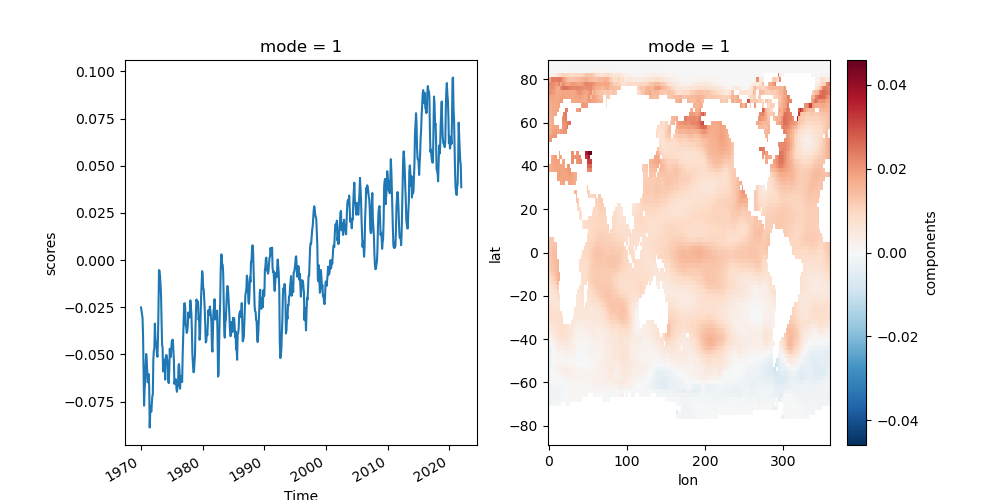
We immediately see that the first mode represents the global warming trend. Yet, the signal is somewhat muddled by short-term and year-to-year variations. Note the pronounced spikes around 1998 and 2016, hinting at the leakage of ENSO signatures into this mode.
fig, ax = plt.subplots(1, 2, figsize=(10, 5))
scores.sel(mode=1).plot(ax=ax[0])
components.sel(mode=1).plot(ax=ax[1])
<matplotlib.collections.QuadMesh object at 0x7f4de4399650>
Now, let’s try to identify this trend more cleanly. To this end, we perform an EEOF analysis on the same data with a suitably large embedding dimension. We choose an embedding dimensioncorresponding to 120 months which is large enough to capture long-term trends. To speed up computation, we apply the EEOF analysis to the extended (lag) covariance matrix derived from the first 50 PCs.
eeof = xe.models.ExtendedEOF(n_modes=5, tau=1, embedding=120, n_pca_modes=50)
eeof.fit(sst, dim="time")
components_ext = eeof.components()
scores_ext = eeof.scores()
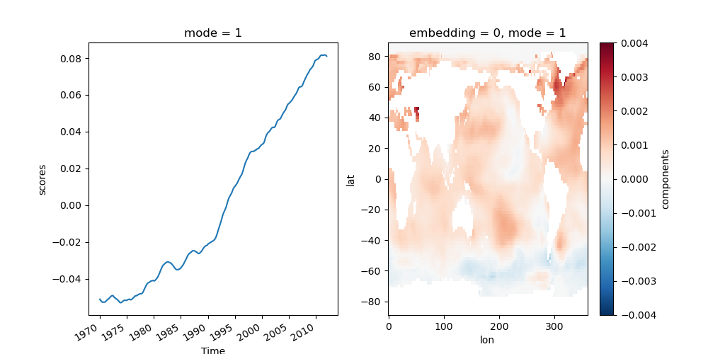
The first mode now represents the global warming trend much more clearly.
fig, ax = plt.subplots(1, 2, figsize=(10, 5))
scores_ext.sel(mode=1).plot(ax=ax[0])
components_ext.sel(mode=1, embedding=0).plot(ax=ax[1])
<matplotlib.collections.QuadMesh object at 0x7f4de3952510>
We can use this to the first mode to remove this nonlinear trend from our original dataset.
sst_trends = eeof.inverse_transform(scores_ext.sel(mode=1))
sst_detrended = sst - sst_trends.drop_vars("mode")
Reapplying the standard EOF analysis on our now detrended dataset:
eof_model_detrended = xe.models.EOF(n_modes=5)
eof_model_detrended.fit(sst_detrended, dim="time")
scores_detrended = eof_model_detrended.scores()
components_detrended = eof_model_detrended.components()
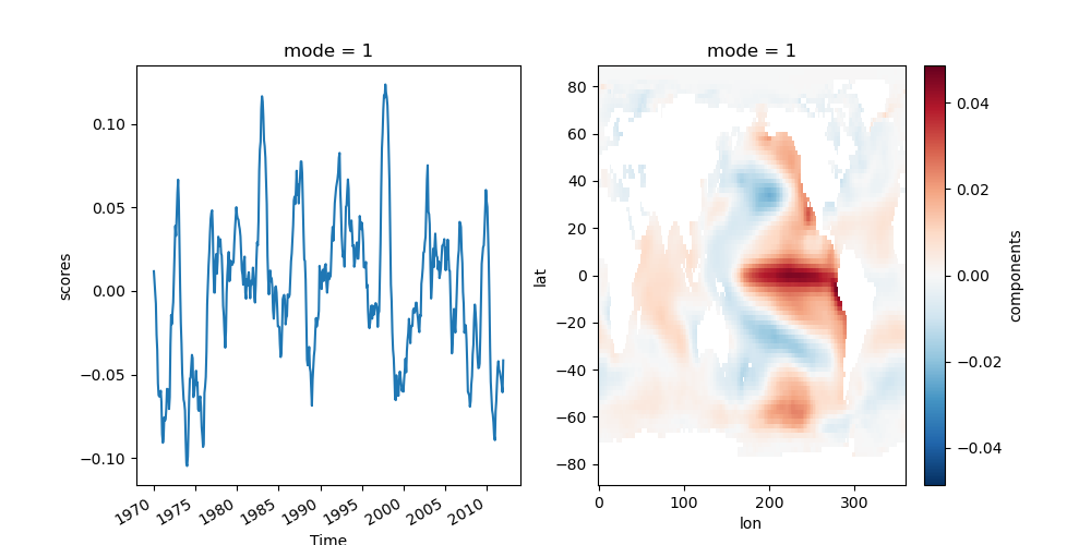
The first mode now represents ENSO without any trend component.
fig, ax = plt.subplots(1, 2, figsize=(10, 5))
scores_detrended.sel(mode=1).plot(ax=ax[0])
components_detrended.sel(mode=1).plot(ax=ax[1])
<matplotlib.collections.QuadMesh object at 0x7f4de32a81d0>
Total running time of the script: (0 minutes 28.072 seconds)