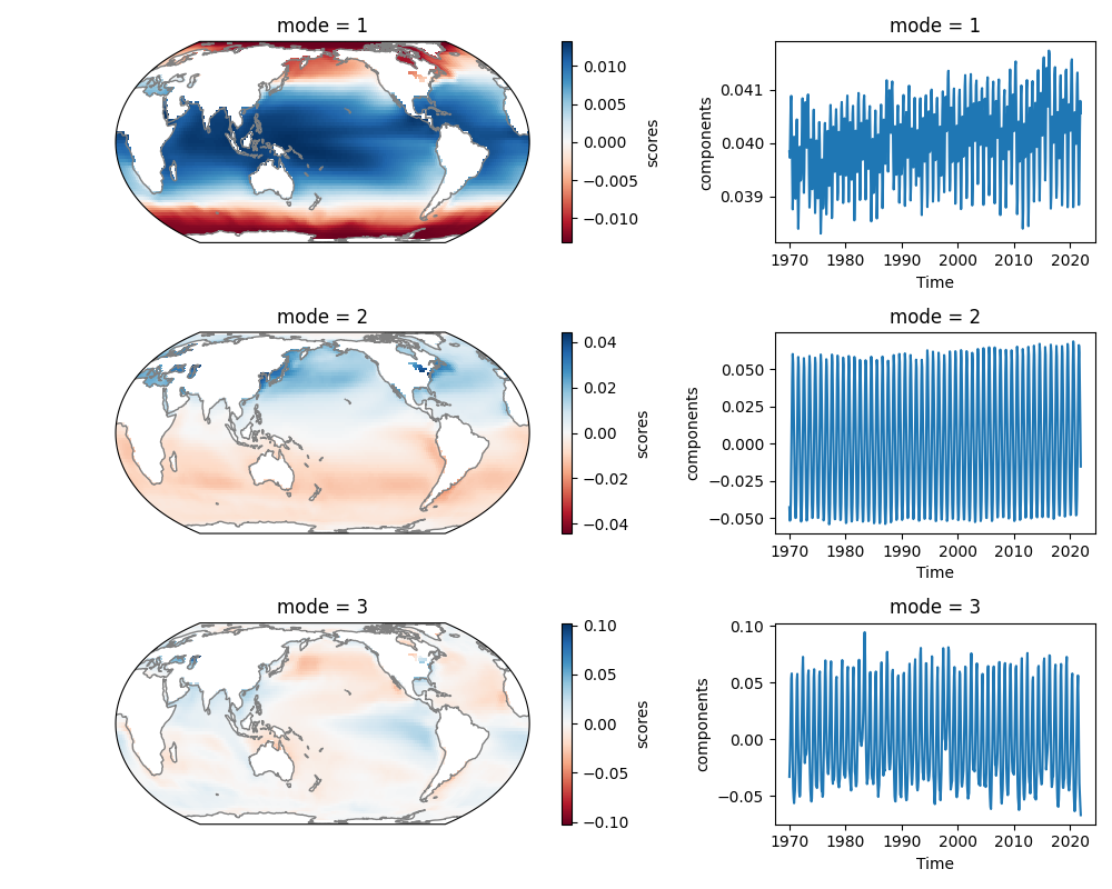
EOF analysis (T-mode)

EOF analysis in T-mode maximises the spatial variance.

Load packages and data:

import xarray as xr
import matplotlib.pyplot as plt
from matplotlib.gridspec import GridSpec
from cartopy.crs import EqualEarth, PlateCarree

from xeofs.models import EOF

sst = xr.tutorial.open_dataset("ersstv5")["sst"]

Perform the actual analysis

model = EOF(n_modes=5)
model.fit(sst, dim=("lat", "lon"))
expvar = model.explained_variance_ratio()
components = model.components()
scores = model.scores()

Create figure showing the first two modes

proj = EqualEarth(central_longitude=180)
kwargs = {"cmap": "RdBu", "transform": PlateCarree()}

fig = plt.figure(figsize=(10, 8))
gs = GridSpec(3, 2, width_ratios=[2, 1])
ax0 = [fig.add_subplot(gs[i, 0], projection=proj) for i in range(3)]
ax1 = [fig.add_subplot(gs[i, 1]) for i in range(3)]

for i, (a0, a1) in enumerate(zip(ax0, ax1)):
    scores.sel(mode=i + 1).plot(ax=a0, **kwargs)
    a0.coastlines(color=".5")
    components.sel(mode=i + 1).plot(ax=a1)

    a0.set_xlabel("")

plt.tight_layout()
plt.savefig("eof-tmode.jpg")