Note
Go to the end to download the full example code
Geographically weighted PCA#
Geographically Weighted Principal Component Analysis (GWPCA) is a spatial analysis method that identifies and visualizes local spatial patterns and relationships in multivariate datasets across various geographic areas. It operates by applying PCA within a moving window over a geographical region, which enables the extraction of local principal components that can differ across locations.
TIn this demonstration, we’ll apply GWPCA to a dataset detailing the chemical compositions of soils from countries around the Baltic Sea [1]. This example is inspired by a tutorial originally crafted and published by Chris Brunsdon [2]. The dataset comprises 10 variables (chemical elements) and spans 768 samples. Here, each sample refers to a pair of latitude and longitude coordinates, representing specific sampling stations.
Note
The dataset we’re using is found in the R package mvoutlier. To access it, we’ll employ the Python package rpy2 which facilitates interaction with R packages from within Python.
Note
Presently, there’s no support for xarray.Dataset lacking an explicit feature dimension.
As a workaround, xarray.DataArray.to_array can be used to convert the Dataset to an DataArray.
Warning
Bear in mind that GWPCA requires significant computational power.
The xeofs implementation is optimized for CPU efficiency and is best suited
for smaller to medium data sets. For more extensive datasets where parallel processing becomes essential,
it’s advisable to turn to the R package GWmodel.
This package harnesses CUDA to enable GPU-accelerated GWPCA for optimized performance.
Let’s import the necessary packages.
# For the analysis
import numpy as np
import xarray as xr
import xeofs as xe

# For visualization
import matplotlib.pyplot as plt
import seaborn as sns

# For accessing R packages
import rpy2.robjects as ro
from rpy2.robjects.packages import importr
from rpy2.robjects import pandas2ri
Next, we’ll install the R package mvoutlier using the rpy2 package.
xr.set_options(display_expand_data=False)
utils = importr("utils")
utils.chooseCRANmirror(ind=1)
utils.install_packages("mvoutlier")
R[write to console]: also installing the dependencies ‘DEoptimR’, ‘sgeostat’, ‘robustbase’


R[write to console]: trying URL 'https://cloud.r-project.org/src/contrib/DEoptimR_1.1-3.tar.gz'

R[write to console]: Content type 'application/x-gzip'
R[write to console]:  length 19222 bytes (18 KB)

R[write to console]: =
R[write to console]: =
R[write to console]: =
R[write to console]: =
R[write to console]: =
R[write to console]: =
R[write to console]: =
R[write to console]: =
R[write to console]: =
R[write to console]: =
R[write to console]: =
R[write to console]: =
R[write to console]: =
R[write to console]: =
R[write to console]: =
R[write to console]: =
R[write to console]: =
R[write to console]: =
R[write to console]: =
R[write to console]: =
R[write to console]: =
R[write to console]: =
R[write to console]: =
R[write to console]: =
R[write to console]: =
R[write to console]: =
R[write to console]: =
R[write to console]: =
R[write to console]: =
R[write to console]: =
R[write to console]: =
R[write to console]: =
R[write to console]: =
R[write to console]: =
R[write to console]: =
R[write to console]: =
R[write to console]: =
R[write to console]: =
R[write to console]: =
R[write to console]: =
R[write to console]: =
R[write to console]: =
R[write to console]: =
R[write to console]: =
R[write to console]: =
R[write to console]: =
R[write to console]: =
R[write to console]: =
R[write to console]: =
R[write to console]: =
R[write to console]:

R[write to console]: downloaded 18 KB


R[write to console]: trying URL 'https://cloud.r-project.org/src/contrib/sgeostat_1.0-27.tar.gz'

R[write to console]: Content type 'application/x-gzip'
R[write to console]:  length 35685 bytes (34 KB)

R[write to console]: =
R[write to console]: =
R[write to console]: =
R[write to console]: =
R[write to console]: =
R[write to console]: =
R[write to console]: =
R[write to console]: =
R[write to console]: =
R[write to console]: =
R[write to console]: =
R[write to console]: =
R[write to console]: =
R[write to console]: =
R[write to console]: =
R[write to console]: =
R[write to console]: =
R[write to console]: =
R[write to console]: =
R[write to console]: =
R[write to console]: =
R[write to console]: =
R[write to console]: =
R[write to console]: =
R[write to console]: =
R[write to console]: =
R[write to console]: =
R[write to console]: =
R[write to console]: =
R[write to console]: =
R[write to console]: =
R[write to console]: =
R[write to console]: =
R[write to console]: =
R[write to console]: =
R[write to console]: =
R[write to console]: =
R[write to console]: =
R[write to console]: =
R[write to console]: =
R[write to console]: =
R[write to console]: =
R[write to console]: =
R[write to console]: =
R[write to console]: =
R[write to console]: =
R[write to console]: =
R[write to console]: =
R[write to console]: =
R[write to console]: =
R[write to console]:

R[write to console]: downloaded 34 KB


R[write to console]: trying URL 'https://cloud.r-project.org/src/contrib/robustbase_0.99-2.tar.gz'

R[write to console]: Content type 'application/x-gzip'
R[write to console]:  length 2292086 bytes (2.2 MB)

R[write to console]: =
R[write to console]: =
R[write to console]: =
R[write to console]: =
R[write to console]: =
R[write to console]: =
R[write to console]: =
R[write to console]: =
R[write to console]: =
R[write to console]: =
R[write to console]: =
R[write to console]: =
R[write to console]: =
R[write to console]: =
R[write to console]: =
R[write to console]: =
R[write to console]: =
R[write to console]: =
R[write to console]: =
R[write to console]: =
R[write to console]: =
R[write to console]: =
R[write to console]: =
R[write to console]: =
R[write to console]: =
R[write to console]: =
R[write to console]: =
R[write to console]: =
R[write to console]: =
R[write to console]: =
R[write to console]: =
R[write to console]: =
R[write to console]: =
R[write to console]: =
R[write to console]: =
R[write to console]: =
R[write to console]: =
R[write to console]: =
R[write to console]: =
R[write to console]: =
R[write to console]: =
R[write to console]: =
R[write to console]: =
R[write to console]: =
R[write to console]: =
R[write to console]: =
R[write to console]: =
R[write to console]: =
R[write to console]: =
R[write to console]: =
R[write to console]:

R[write to console]: downloaded 2.2 MB


R[write to console]: trying URL 'https://cloud.r-project.org/src/contrib/mvoutlier_2.1.1.tar.gz'

R[write to console]: Content type 'application/x-gzip'
R[write to console]:  length 476636 bytes (465 KB)

R[write to console]: =
R[write to console]: =
R[write to console]: =
R[write to console]: =
R[write to console]: =
R[write to console]: =
R[write to console]: =
R[write to console]: =
R[write to console]: =
R[write to console]: =
R[write to console]: =
R[write to console]: =
R[write to console]: =
R[write to console]: =
R[write to console]: =
R[write to console]: =
R[write to console]: =
R[write to console]: =
R[write to console]: =
R[write to console]: =
R[write to console]: =
R[write to console]: =
R[write to console]: =
R[write to console]: =
R[write to console]: =
R[write to console]: =
R[write to console]: =
R[write to console]: =
R[write to console]: =
R[write to console]: =
R[write to console]: =
R[write to console]: =
R[write to console]: =
R[write to console]: =
R[write to console]: =
R[write to console]: =
R[write to console]: =
R[write to console]: =
R[write to console]: =
R[write to console]: =
R[write to console]: =
R[write to console]: =
R[write to console]: =
R[write to console]: =
R[write to console]: =
R[write to console]: =
R[write to console]: =
R[write to console]: =
R[write to console]: =
R[write to console]: =
R[write to console]:

R[write to console]: downloaded 465 KB


R[write to console]:

R[write to console]:
R[write to console]: The downloaded source packages are in
        ‘/tmp/Rtmpr8iXHn/downloaded_packages’
R[write to console]:
R[write to console]:

R[write to console]: Updating HTML index of packages in '.Library'

R[write to console]: Making 'packages.html' ...
R[write to console]:  done


<rpy2.rinterface_lib.sexp.NULLType object at 0x7fa747af2890> [0]
Let’s load the dataset and convert it into a pandas.DataFrame.
Alongside, we’ll also load the background data that outlines the borders of countries
in the Baltic Sea region. This will help us visually represent the GWPCA results.
ro.r(
    """
    require("mvoutlier")
    data(bsstop)
    Data <- bsstop[,1:14]
    background <- bss.background
    """
)
with (ro.default_converter + pandas2ri.converter).context():
    data_df = ro.conversion.get_conversion().rpy2py(ro.r["Data"])
    background_df = ro.conversion.get_conversion().rpy2py(ro.r["background"])
data_df.head()
R[write to console]: Loading required package: mvoutlier

R[write to console]: Loading required package: sgeostat
Since xeofs uses xarray, we convert the data into an xarray.DataArray.
data_df = data_df.rename(columns={"ID": "station"}).set_index("station")
data = data_df.to_xarray()
data = data.rename({"XCOO": "x", "YCOO": "y"})
data = data.set_index(station=("x", "y"))
data = data.drop_vars("CNo")
da = data.to_array(dim="element")
da
Let’s dive into the GWPCA. First, initialize a GWPCA instance and fit it to the data.
The station dimension serves as our sample dimension, along which the local PCAs will be applied.
Since these PCAs need to gauge distances to adjacent stations, we must specify
a distance metric. Our station data includes coordinates in meters, so we’ll
choose the euclidean metric. If you have coordinates in degrees (like
latitude and longitude), choose the haversine metric instead.
We’re also using a bisquare kernel with a bandwidth of 1000 km. Note that the
bandwidth unit always follows input data (which is in meters here),
except when using the haversine metric, which always gives distances in
kilometers. Lastly, we’ll standardize the input to ensure consistent scales
for the chemical elements.
gwpca = xe.models.GWPCA(
    n_modes=5,
    standardize=True,
    metric="euclidean",
    kernel="bisquare",
    bandwidth=1000000.0,
)
gwpca.fit(da, "station")
gwpca.components()
The components method returns the local principal components for each station. Note that the
dimensionality of the returned array is [station, element, mode], so in practice we don’t really have
reduced the dimensionality of the data set. However, we can
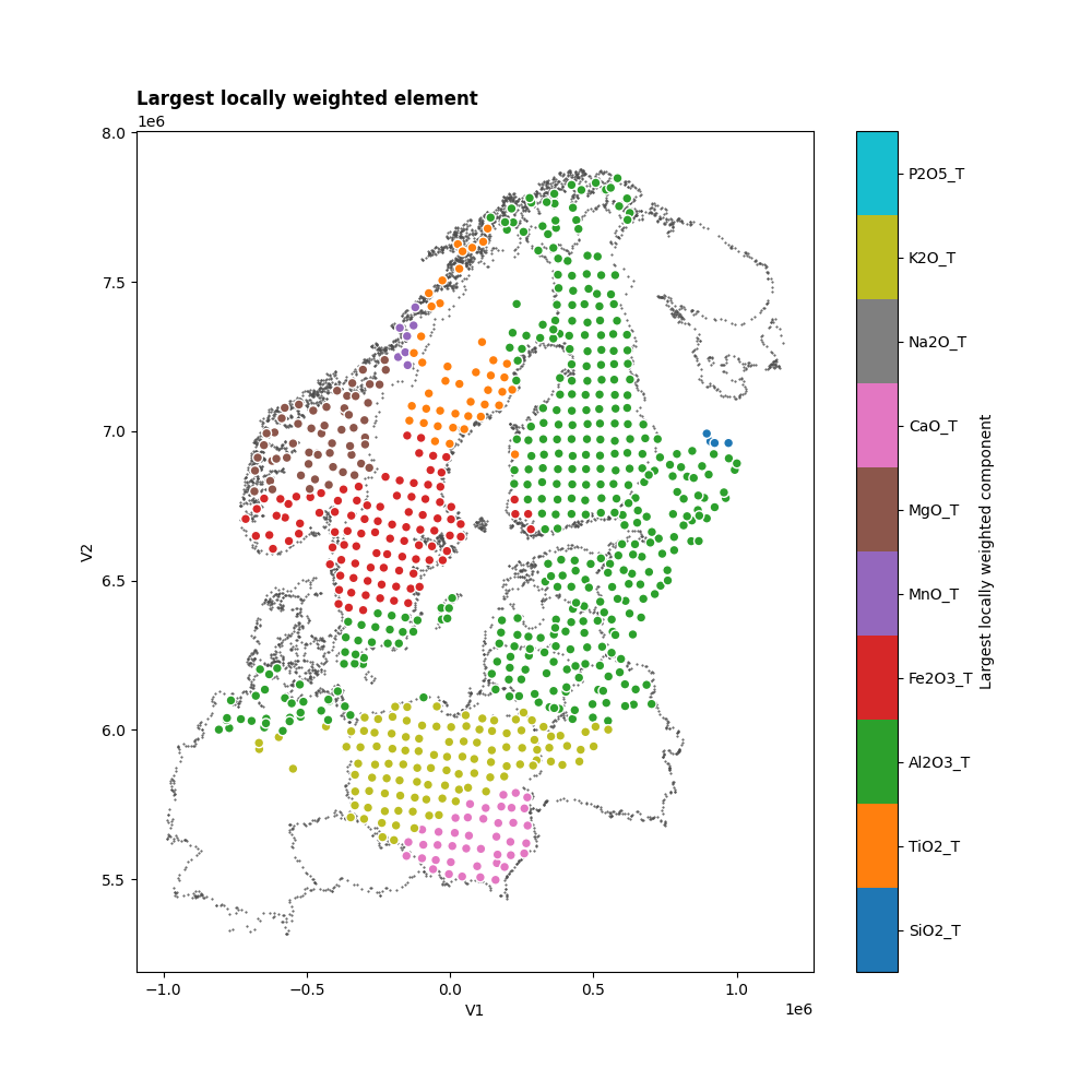
extract the largest locally weighted components for each station which tells us which chemical elements
dominate the local PCAs.
llwc = gwpca.largest_locally_weighted_components()
llwc
Let’s visualize the spatial patterns of the chemical elements.
As the stations are positioned on a irregular grid, we’ll transform the
llwc DataArray into a pandas.DataFrame. After that, we can easily visualize
it using the scatter method.
For demonstation, we’ll concentrate on the first mode:
llwc1_df = llwc.sel(mode=1).to_dataframe()

elements = da.element.values
n_elements = len(elements)
colors = np.arange(n_elements)
col_dict = {el: col for el, col in zip(elements, colors)}

llwc1_df["colors"] = llwc1_df["largest_locally_weighted_components"].map(col_dict)
cmap = sns.color_palette("tab10", n_colors=n_elements, as_cmap=True)


fig = plt.figure(figsize=(10, 10))
ax = fig.add_subplot(111)
background_df.plot.scatter(ax=ax, x="V1", y="V2", color=".3", marker=".", s=1)
s = ax.scatter(
    x=llwc1_df["x"],
    y=llwc1_df["y"],
    c=llwc1_df["colors"],
    ec="w",
    s=40,
    cmap=cmap,
    vmin=-0.5,
    vmax=n_elements - 0.5,
)
cbar = fig.colorbar(mappable=s, ax=ax, label="Largest locally weighted component")
cbar.set_ticks(colors)
cbar.set_ticklabels(elements)
ax.set_title("Largest locally weighted element", loc="left", weight=800)
plt.show()
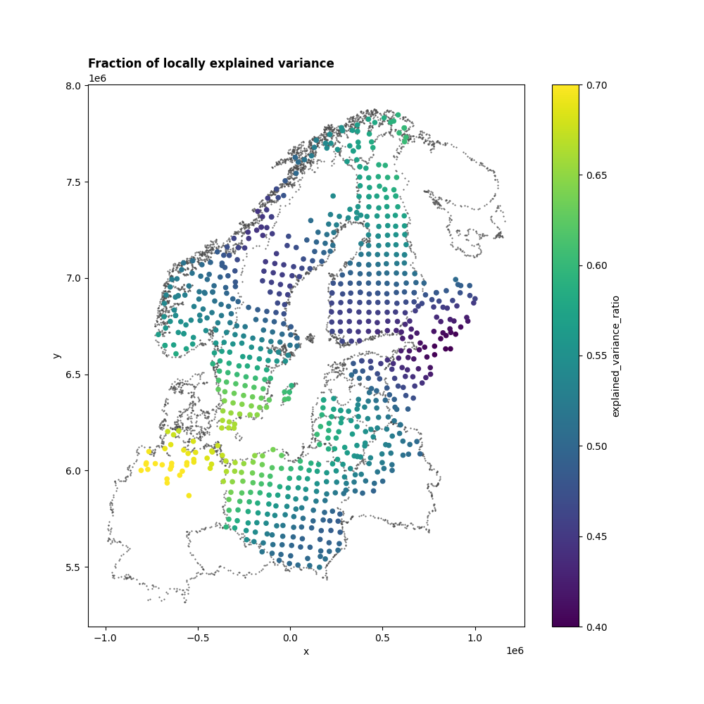
In the final step, let’s examine the explained variance. Like standard PCA, this gives us insight into the variance explained by each mode. But with a local PCA for every station, the explained variance varies spatially. Notably, the first mode’s explained variance differs across countries, ranging from roughly 40% to 70%.
exp_var_ratio = gwpca.explained_variance_ratio()
evr1_df = exp_var_ratio.sel(mode=1).to_dataframe()

fig = plt.figure(figsize=(10, 10))
ax = fig.add_subplot(111)
background_df.plot.scatter(ax=ax, x="V1", y="V2", color=".3", marker=".", s=1)
evr1_df.plot.scatter(
    ax=ax, x="x", y="y", c="explained_variance_ratio", vmin=0.4, vmax=0.7
)
ax.set_title("Fraction of locally explained variance", loc="left", weight=800)
plt.show()
Total running time of the script: (0 minutes 34.593 seconds)