Note
Go to the end to download the full example code
Extented EOF analysis#
This example demonstrates Extended EOF (EEOF) analysis on xarray tutorial
data. EEOF analysis, also termed as Multivariate/Multichannel Singular
Spectrum Analysis, advances traditional EOF analysis to capture propagating
signals or oscillations in multivariate datasets. At its core, this
involves the formulation of a lagged covariance matrix that encapsulates
both spatial and temporal correlations. Subsequently, this matrix is
decomposed to yield its eigenvectors (components) and eigenvalues (explained variance).
Let’s begin by setting up the required packages and fetching the data:
import xarray as xr
import xeofs as xe
import matplotlib.pyplot as plt

xr.set_options(display_expand_data=False)
<xarray.core.options.set_options object at 0x7ffac7efbc10>
Load the tutorial data.
t2m = xr.tutorial.load_dataset("air_temperature").air
Prior to conducting the EEOF analysis, it’s essential to determine the
structure of the lagged covariance matrix. This entails defining the time
delay tau and the embedding dimension. The former signifies the
interval between the original and lagged time series, while the latter
dictates the number of time-lagged copies in the delay-coordinate space,
representing the system’s dynamics.
For illustration, using tau=4 and embedding=40, we generate 40
delayed versions of the time series, each offset by 4 time steps, resulting
in a maximum shift of tau x embedding = 160. Given our dataset’s
6-hour intervals, tau = 4 translates to a 24-hour shift.
It’s obvious that this way of constructing the lagged covariance matrix
and subsequently decomposing it can be computationally expensive. For example,
given our dataset’s dimensions,
t2m.shape
(2920, 25, 53)
the extended dataset would have 40 x 25 x 53 = 53000 features
which is much larger than the original dataset’s 1325 features.
To mitigate this, we can first preprocess the data using PCA / EOF analysis
and then perform EEOF analysis on the resulting PCA / EOF scores. Here,
we’ll use n_pca_modes=50 to retain the first 50 PCA modes, so we end
up with 40 x 50 = 200 (latent) features.
With these parameters set, we proceed to instantiate the ExtendedEOF
model and fit our data.
model = xe.models.ExtendedEOF(
    n_modes=10, tau=4, embedding=40, n_pca_modes=50, use_coslat=True
)
model.fit(t2m, dim="time")
scores = model.scores()
components = model.components()
components
A notable distinction from standard EOF analysis is the incorporation of an
extra embedding dimension in the components. Nonetheless, the
overarching methodology mirrors traditional EOF practices. The results,
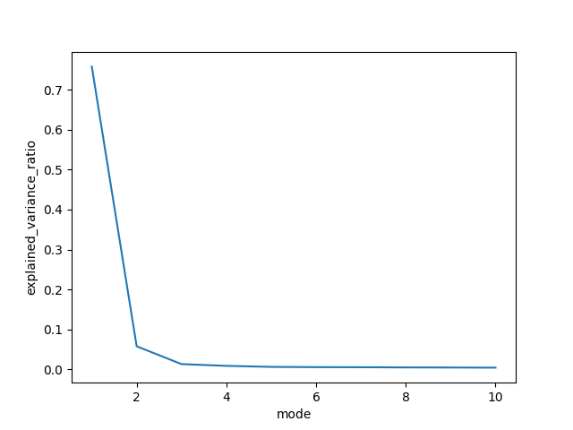
for instance, can be assessed by examining the explained variance ratio.
model.explained_variance_ratio().plot()
plt.show()
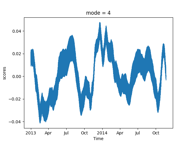
Additionally, we can look into the scores; let’s spotlight mode 4.
scores.sel(mode=4).plot()
plt.show()
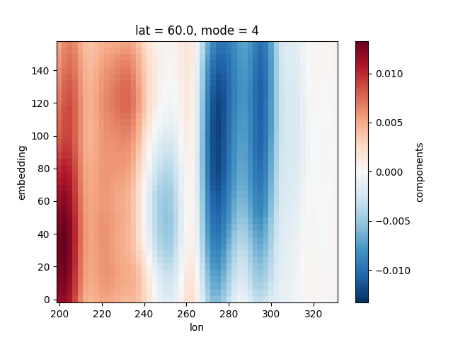
In wrapping up, we visualize the corresponding EEOF component of mode 4. For visualization purposes, we’ll focus on the component at a specific latitude, in this instance, 60 degrees north.
components.sel(mode=4, lat=60).plot()
plt.show()
Total running time of the script: (0 minutes 0.777 seconds)