Rotated EOF analysis

EOF (Empirical Orthogonal Function) analysis is commonly used in climate science, interpreting the derived eigenvectors (EOFs) as climatic variability patterns. However, due to the inherent orthogonality constraint in EOF analysis, the interpretation of all but the first EOF can be problematic. Rotated EOF analysis, using optimization criteria like Varimax and Promax, offers a solution by releasing this orthogonality constraint, thus enabling a more accurate interpretation of variability patterns.

Both Varimax (orthogonal) and Promax (oblique) rotations result in “sparse” solutions, meaning the EOFs become more interpretable by limiting the number of variables that contribute to each EOF. This rotation effectively serves as a regularization method for the EOF solution, with the strength of regularization determined by the power parameter; the higher the value, the sparser the EOFs.

Promax rotation, with a small regularization value (i.e., power=1), reverts to Varimax rotation. In this context, we compare the first three modes of EOF analysis: (1) without regularization, (2) with Varimax rotation, and (3) with Promax rotation.

We’ll start by loading the necessary packages and data:

import xarray as xr
import matplotlib.pyplot as plt
import seaborn as sns
from matplotlib.gridspec import GridSpec
from cartopy.crs import Robinson, PlateCarree

from xeofs.models import EOF, EOFRotator


sns.set_context("paper")

sst = xr.tutorial.open_dataset("ersstv5")["sst"]

Perform the actual analysis

components = []
scores = []
# (1) Standard EOF without regularization
model = EOF(n_modes=100, standardize=True, use_coslat=True)
model.fit(sst, dim="time")
components.append(model.components())
scores.append(model.scores())
# (2) Varimax-rotated EOF analysis
rot_var = EOFRotator(n_modes=50, power=1)
rot_var.fit(model)
components.append(rot_var.components())
scores.append(rot_var.scores())
# (3) Promax-rotated EOF analysis
rot_pro = EOFRotator(n_modes=50, power=4)
rot_pro.fit(model)
components.append(rot_pro.components())
scores.append(rot_pro.scores())

/home/slevang/miniconda3/envs/xeofs-docs/lib/python3.11/site-packages/numpy/lib/nanfunctions.py:1879: RuntimeWarning: Degrees of freedom <= 0 for slice.
  var = nanvar(a, axis=axis, dtype=dtype, out=out, ddof=ddof,

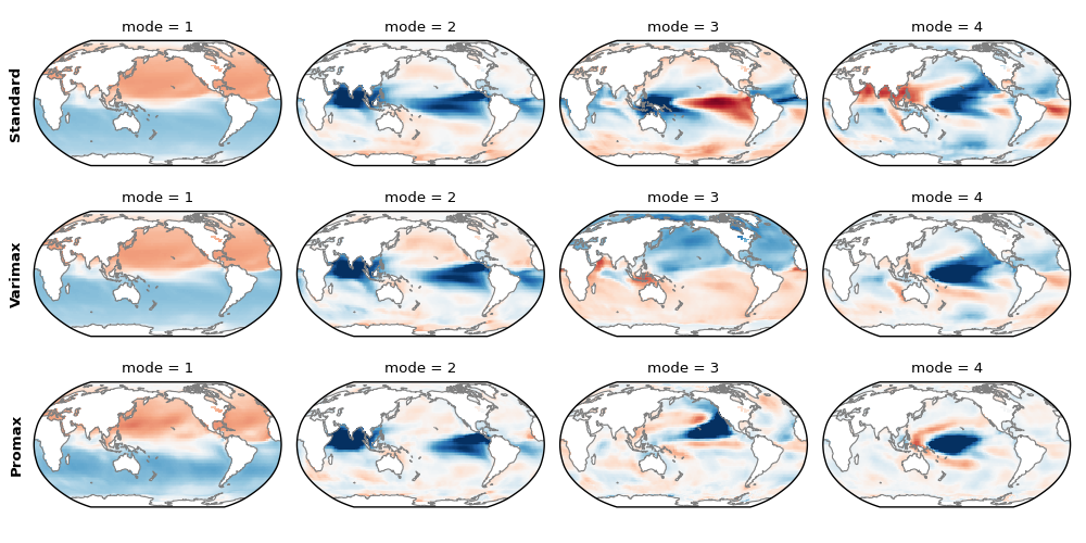
Create figure showing the first 6 modes for all 3 cases. While the first mode is very similar in all three cases the subsequent modes of the standard solution exhibit dipole and tripole-like patterns. Under Varimax and Promax rotation, these structures completely disappear suggesting that these patterns were mere artifacts due to the orthogonality.

proj = Robinson(central_longitude=180)
kwargs = {
    "cmap": "RdBu",
    "transform": PlateCarree(),
    "vmin": -0.03,
    "vmax": +0.03,
    "add_colorbar": False,
}

fig = plt.figure(figsize=(10, 5))
gs = GridSpec(3, 4)
ax_std = [fig.add_subplot(gs[0, i], projection=proj) for i in range(4)]
ax_var = [fig.add_subplot(gs[1, i], projection=proj) for i in range(4)]
ax_pro = [fig.add_subplot(gs[2, i], projection=proj) for i in range(4)]

for i, (a0, a1, a2) in enumerate(zip(ax_std, ax_var, ax_pro)):
    mode = i + 1
    a0.coastlines(color=".5")
    a1.coastlines(color=".5")
    a2.coastlines(color=".5")
    components[0].sel(mode=mode).plot(ax=a0, **kwargs)
    components[1].sel(mode=mode).plot(ax=a1, **kwargs)
    components[2].sel(mode=mode).plot(ax=a2, **kwargs)

title_kwargs = dict(rotation=90, va="center", weight="bold")
ax_std[0].text(-0.1, 0.5, "Standard", transform=ax_std[0].transAxes, **title_kwargs)
ax_var[0].text(-0.1, 0.5, "Varimax", transform=ax_var[0].transAxes, **title_kwargs)
ax_pro[0].text(-0.1, 0.5, "Promax", transform=ax_pro[0].transAxes, **title_kwargs)

plt.tight_layout()
plt.savefig("rotated_eof.jpg", dpi=200)