Canonical Correlation Analysis

In this example, we’re going to perform a Canonical Correlation Analysis (CCA) on three datasets using the ERSSTv5 monthly sea surface temperature (SST) data from 1970 to 2022. We divide this data into three areas: the Indian Ocean, the Pacific Ocean, and the Atlantic Ocean. Our goal is to perform CCA on these regions.

First, we’ll import the necessary modules.

import xarray as xr
import xeofs as xe

import matplotlib.pyplot as plt
from matplotlib.gridspec import GridSpec
import cartopy.crs as ccrs

Next, we load the data and compute the SST anomalies. This removes the monthly climatologies, so the seasonal cycle doesn’t impact our CCA.

sst = xr.tutorial.load_dataset("ersstv5").sst
sst = sst.groupby("time.month") - sst.groupby("time.month").mean("time")

Now, we define the three regions of interest and store them in a list.

indian = sst.sel(lon=slice(35, 115), lat=slice(30, -30))
pacific = sst.sel(lon=slice(130, 290), lat=slice(30, -30))
atlantic = sst.sel(lon=slice(320, 360), lat=slice(70, 10))

data_list = [indian, pacific, atlantic]

We now perform CCA. Since we are dealing with a high-dimensional feature space, we first perform PCA to reduce the dimensionality (this is kind of a regularized CCA) by setting pca=True. By setting the variance_fraction keyword argument, we specify that we want to keep the number of PCA modes that explain 90% of the variance in each of the three data sets.

An important parameter is init_pca_modes. It specifies the number of PCA modes that are initially compute before truncating them to account for 90 %. If this number is small enough, randomized PCAs will be performed instead of the full SVD decomposition which is much faster. We can also specify init_pca_modes as a float (0 < x <= 1), in which case the number of PCA modes is given by the fraction of the data matrix’s rank The default is set to 0.75 which will ensure that randomized PCAs are performed.

Given the nature of SST data, we might lower it to something like 0.3, since we expect that most of the variance in the data will be explained by a small number of PC modes.

Note that if our initial PCA modes don’t hit the 90% variance target, xeofs will give a warning.

model = xe.models.CCA(
    n_modes=2,
    use_coslat=True,
    pca=True,
    variance_fraction=0.9,
    init_pca_modes=0.30,
)
model.fit(data_list, dim="time")
components = model.components()
scores = model.scores()

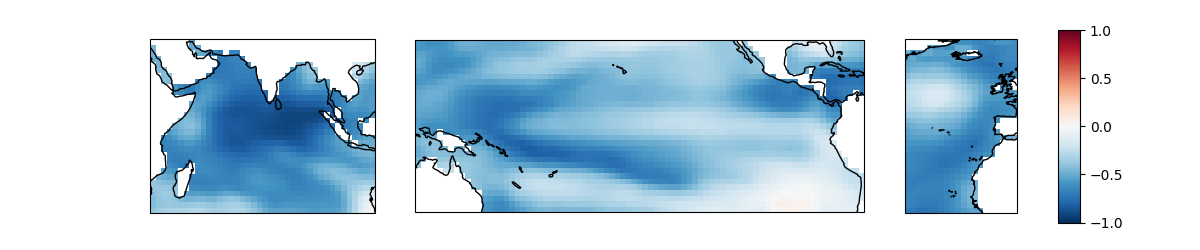
Let’s look at the canonical loadings (components) of the first mode.

mode = 1

central_longitudes = [
    indian.lon.median().item(),
    pacific.lon.median().item(),
    pacific.lon.median().item(),
]
projections = [ccrs.PlateCarree(central_longitude=lon) for lon in central_longitudes]

fig = plt.figure(figsize=(12, 2.5))
gs = GridSpec(1, 4, figure=fig, width_ratios=[2, 4, 1, 0.2])
axes = [fig.add_subplot(gs[0, i], projection=projections[i]) for i in range(3)]
cax = fig.add_subplot(1, 4, 4)
kwargs = dict(transform=ccrs.PlateCarree(), vmin=-1, vmax=1, cmap="RdBu_r", cbar_ax=cax)
components[0].sel(mode=mode).plot(ax=axes[0], **kwargs)
components[1].sel(mode=mode).plot(ax=axes[1], **kwargs)
im = components[2].sel(mode=mode).plot(ax=axes[2], **kwargs)
fig.colorbar(im, cax=cax, orientation="vertical")
for ax in axes:
    ax.coastlines()
    ax.set_title("")

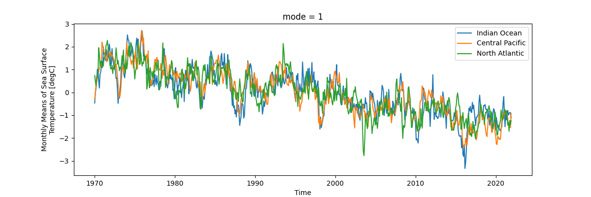
And lastly, we’ll check out the canonical variates (scores) of the first mode.

fig, ax = plt.subplots(figsize=(12, 4))
scores[0].sel(mode=mode).plot(ax=ax, label="Indian Ocean")
scores[1].sel(mode=mode).plot(ax=ax, label="Central Pacific")
scores[2].sel(mode=mode).plot(ax=ax, label="North Atlantic")
ax.legend()

<matplotlib.legend.Legend object at 0x7fa6fa2bb3d0>