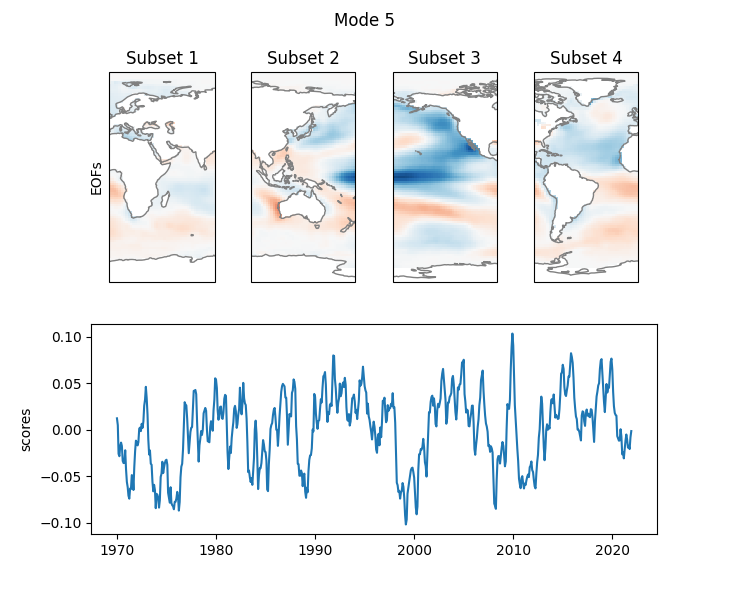
Varimax-rotated Multivariate EOF analysis

Multivariate EOF analysis with additional Varimax rotation.

# Load packages and data:
import xarray as xr
import matplotlib.pyplot as plt
from matplotlib.gridspec import GridSpec
from cartopy.crs import PlateCarree

from xeofs.models import EOF, EOFRotator

Create four different dataarrayss

sst = xr.tutorial.open_dataset("ersstv5")["sst"]
subset1 = sst.isel(lon=slice(0, 45))
subset2 = sst.isel(lon=slice(46, 90))
subset3 = sst.isel(lon=slice(91, 135))
subset4 = sst.isel(lon=slice(136, None))

Perform the actual analysis

multivariate_data = [subset1, subset2, subset3, subset4]
mpca = EOF(n_modes=100, standardize=False, use_coslat=True)
mpca.fit(multivariate_data, dim="time")
rotator = EOFRotator(n_modes=20)
rotator.fit(mpca)
rcomponents = rotator.components()
rscores = rotator.scores()

Plot mode 1

mode = 5
proj = PlateCarree()
kwargs = {
    "cmap": "RdBu",
    "vmin": -0.05,
    "vmax": 0.05,
    "transform": proj,
    "add_colorbar": False,
}

fig = plt.figure(figsize=(7.3, 6))
fig.subplots_adjust(wspace=0)
gs = GridSpec(2, 4, figure=fig, width_ratios=[1, 1, 1, 1])
ax = [fig.add_subplot(gs[0, i], projection=proj) for i in range(4)]
ax_pc = fig.add_subplot(gs[1, :])

# PC
rscores.sel(mode=mode).plot(ax=ax_pc)
ax_pc.set_xlabel("")
ax_pc.set_title("")

# EOFs
for i, (a, comps) in enumerate(zip(ax, rcomponents)):
    a.coastlines(color=".5")
    comps.sel(mode=mode).plot(ax=a, **kwargs)
    a.set_xticks([], [])
    a.set_yticks([], [])
    a.set_xlabel("")
    a.set_ylabel("")
    a.set_title("Subset {:}".format(i + 1))
ax[0].set_ylabel("EOFs")
fig.suptitle("Mode {:}".format(mode))
plt.savefig("mreof-analysis.jpg")