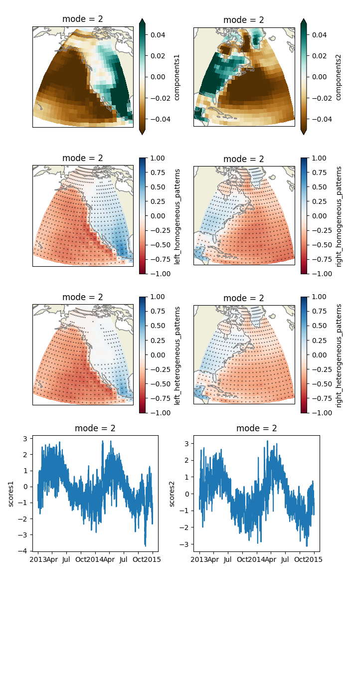
Maximum Covariance Analysis

Maximum Covariance Analysis (MCA) between two data sets.

# Load packages and data:
import numpy as np
import xarray as xr
import matplotlib.pyplot as plt
from matplotlib.gridspec import GridSpec
from cartopy.crs import Orthographic, PlateCarree
from cartopy.feature import LAND

from xeofs.models import MCA

Create 2 different DataArrays

t2m = xr.tutorial.load_dataset("air_temperature")["air"]
da1 = t2m.isel(lon=slice(0, 26))
da2 = t2m.isel(lon=slice(27, None))

Perform MCA

mca = MCA(n_modes=20, standardize=False, use_coslat=True)
mca.fit(da1, da2, dim="time")

<xeofs.models.mca.MCA object at 0x7fa6f9db1d50>

Get singular vectors, projections (PCs), homogeneous and heterogeneous patterns:

singular_vectors = mca.components()
scores = mca.scores()
hom_pats, pvals_hom = mca.homogeneous_patterns()
het_pats, pvals_het = mca.heterogeneous_patterns()

When two fields are expected, the output of the above methods is a list of length 2, with the first and second entry containing the relevant object for X and Y. For example, the p-values obtained from the two-sided t-test for the homogeneous patterns of X are:

pvals_hom[0]

<xarray.DataArray 'pvalues_of_left_homogeneous_patterns' (mode: 20, lat: 25,
                                                          lon: 26)> Size: 104kB
7.302e-298 4.926e-268 8.327e-265 3.64e-251 ... 0.04256 0.08683 0.1689 0.2897
Coordinates:
  * lat      (lat) float32 100B 15.0 17.5 20.0 22.5 25.0 ... 67.5 70.0 72.5 75.0
  * lon      (lon) float32 104B 200.0 202.5 205.0 207.5 ... 257.5 260.0 262.5
  * mode     (mode) int64 160B 1 2 3 4 5 6 7 8 9 ... 12 13 14 15 16 17 18 19 20
Attributes: (12/16)
    model:          MCA
    software:       xeofs
    version:        2.3.2
    date:           2024-03-31 21:13:25
    n_modes:        20
    center:         True
    ...             ...
    compute:        True
    sample_name:    sample
    feature_name:   feature
    solver:         auto
    random_state:   None
    solver_kwargs:  {}

xarray.DataArray

'pvalues_of_left_homogeneous_patterns'

• mode: 20
• lat: 25
• lon: 26

• 7.302e-298 4.926e-268 8.327e-265 3.64e-251 ... 0.08683 0.1689 0.2897

  array([[[7.30218548e-298, 4.92608968e-268, 8.32666599e-265, ...,
           1.08710962e-108, 1.03682895e-164, 0.00000000e+000],
          [0.00000000e+000, 1.11101678e-316, 1.20739041e-261, ...,
           4.10556693e-131, 1.44386567e-128, 2.12643490e-154],
          [0.00000000e+000, 0.00000000e+000, 3.62977382e-317, ...,
           7.98272642e-039, 2.30418635e-094, 2.21467374e-303],
          ...,
          [0.00000000e+000, 0.00000000e+000, 0.00000000e+000, ...,
           0.00000000e+000, 0.00000000e+000, 0.00000000e+000],
          [0.00000000e+000, 0.00000000e+000, 0.00000000e+000, ...,
           0.00000000e+000, 0.00000000e+000, 0.00000000e+000],
          [0.00000000e+000, 0.00000000e+000, 0.00000000e+000, ...,
           0.00000000e+000, 0.00000000e+000, 0.00000000e+000]],
  
         [[3.53253635e-053, 2.16418457e-064, 1.82052734e-072, ...,
           2.73858136e-061, 1.91558844e-001, 1.78817478e-051],
          [1.09096681e-048, 9.62776394e-054, 5.03544401e-061, ...,
           5.32170507e-062, 3.17685659e-139, 4.93127028e-125],
          [2.28491441e-026, 6.67760144e-023, 1.31644526e-042, ...,
           3.45657054e-301, 5.93584867e-211, 6.80859724e-056],
  ...
          [6.67998378e-015, 6.36747968e-016, 1.40411398e-015, ...,
           7.79516123e-001, 5.47945593e-001, 3.94367920e-001],
          [1.60490441e-010, 2.56600869e-010, 1.28088604e-009, ...,
           2.29172125e-001, 1.46246686e-001, 1.06877734e-001],
          [1.32439970e-009, 3.66361534e-009, 1.85905814e-008, ...,
           1.67861191e-001, 1.50369648e-001, 1.54502185e-001]],
  
         [[3.52372539e-001, 1.68753186e-002, 1.89053645e-002, ...,
           7.85244066e-001, 2.77742777e-004, 2.09288327e-009],
          [3.51869929e-001, 2.03883160e-001, 1.77938328e-001, ...,
           1.67776720e-003, 1.75502701e-004, 3.62721492e-006],
          [4.94676985e-001, 3.67658066e-001, 1.12714727e-001, ...,
           1.02155538e-007, 7.09176181e-005, 3.77178517e-004],
          ...,
          [4.03302319e-019, 1.70922676e-018, 2.01737186e-017, ...,
           6.53897033e-001, 6.06527999e-001, 5.74043314e-001],
          [7.99228849e-007, 2.85889857e-006, 1.07502551e-005, ...,
           8.18001986e-001, 9.27700759e-001, 9.60585386e-001],
          [3.44012356e-002, 6.48368282e-002, 1.22449592e-001, ...,
           8.68256087e-002, 1.68872024e-001, 2.89727071e-001]]])

• Coordinates: (3)
  • lat
    (lat)
    float32
    15.0 17.5 20.0 ... 70.0 72.5 75.0

    array([15. , 17.5, 20. , 22.5, 25. , 27.5, 30. , 32.5, 35. , 37.5, 40. , 42.5,
           45. , 47.5, 50. , 52.5, 55. , 57.5, 60. , 62.5, 65. , 67.5, 70. , 72.5,
           75. ], dtype=float32)

  • lon
    (lon)
    float32
    200.0 202.5 205.0 ... 260.0 262.5

    array([200. , 202.5, 205. , 207.5, 210. , 212.5, 215. , 217.5, 220. , 222.5,
           225. , 227.5, 230. , 232.5, 235. , 237.5, 240. , 242.5, 245. , 247.5,
           250. , 252.5, 255. , 257.5, 260. , 262.5], dtype=float32)

  • mode
    (mode)
    int64
    1 2 3 4 5 6 7 ... 15 16 17 18 19 20

    array([ 1,  2,  3,  4,  5,  6,  7,  8,  9, 10, 11, 12, 13, 14, 15, 16, 17, 18,
           19, 20])

• Indexes: (3)
  • mode
    PandasIndex

    PandasIndex(Index([1, 2, 3, 4, 5, 6, 7, 8, 9, 10, 11, 12, 13, 14, 15, 16, 17, 18, 19, 20], dtype='int64', name='mode'))

  • lat
    PandasIndex

    PandasIndex(Index([15.0, 17.5, 20.0, 22.5, 25.0, 27.5, 30.0, 32.5, 35.0, 37.5, 40.0, 42.5,
           45.0, 47.5, 50.0, 52.5, 55.0, 57.5, 60.0, 62.5, 65.0, 67.5, 70.0, 72.5,
           75.0],
          dtype='float32', name='lat'))

  • lon
    PandasIndex

    PandasIndex(Index([200.0, 202.5, 205.0, 207.5, 210.0, 212.5, 215.0, 217.5, 220.0, 222.5,
           225.0, 227.5, 230.0, 232.5, 235.0, 237.5, 240.0, 242.5, 245.0, 247.5,
           250.0, 252.5, 255.0, 257.5, 260.0, 262.5],
          dtype='float32', name='lon'))

• Attributes: (16)

  model :

  MCA

  software :

  xeofs

  version :

  2.3.2

  date :

  2024-03-31 21:13:25

  n_modes :

  20

  center :

  True

  standardize :

  False

  use_coslat :

  True

  check_nans :

  True

  n_pca_modes :

  None

  compute :

  True

  sample_name :

  sample

  feature_name :

  feature

  solver :

  auto

  random_state :

  None

  solver_kwargs :

  {}

Create a mask to identifiy where p-values are below 0.05

hom_mask = [values < 0.05 for values in pvals_hom]
het_mask = [values < 0.05 for values in pvals_het]

Plot some relevant quantities of mode 2.

lonlats = [
    np.meshgrid(pvals_hom[0].lon.values, pvals_hom[0].lat.values),
    np.meshgrid(pvals_hom[1].lon.values, pvals_hom[1].lat.values),
]
proj = [
    Orthographic(central_latitude=30, central_longitude=-120),
    Orthographic(central_latitude=30, central_longitude=-60),
]
kwargs1 = {"cmap": "BrBG", "vmin": -0.05, "vmax": 0.05, "transform": PlateCarree()}
kwargs2 = {"cmap": "RdBu", "vmin": -1, "vmax": 1, "transform": PlateCarree()}

mode = 2

fig = plt.figure(figsize=(7, 14))
gs = GridSpec(5, 2)
ax1 = [fig.add_subplot(gs[0, i], projection=proj[i]) for i in range(2)]
ax2 = [fig.add_subplot(gs[1, i], projection=proj[i]) for i in range(2)]
ax3 = [fig.add_subplot(gs[2, i], projection=proj[i]) for i in range(2)]
ax4 = [fig.add_subplot(gs[3, i]) for i in range(2)]

for i, a in enumerate(ax1):
    singular_vectors[i].sel(mode=mode).plot(ax=a, **kwargs1)

for i, a in enumerate(ax2):
    hom_pats[i].sel(mode=mode).plot(ax=a, **kwargs2)
    a.scatter(
        lonlats[i][0],
        lonlats[i][1],
        hom_mask[i].sel(mode=mode).values * 0.5,
        color="k",
        alpha=0.5,
        transform=PlateCarree(),
    )
for i, a in enumerate(ax3):
    het_pats[i].sel(mode=mode).plot(ax=a, **kwargs2)
    a.scatter(
        lonlats[i][0],
        lonlats[i][1],
        het_mask[i].sel(mode=mode).values * 0.5,
        color="k",
        alpha=0.5,
        transform=PlateCarree(),
    )

for i, a in enumerate(ax4):
    scores[i].sel(mode=mode).plot(ax=a)
    a.set_xlabel("")


for a in np.ravel([ax1, ax2, ax3]):
    a.coastlines(color=".5")
    a.add_feature(LAND)

plt.tight_layout()
plt.savefig("mca.jpg")

/home/slevang/miniconda3/envs/xeofs-docs/lib/python3.11/site-packages/cartopy/io/__init__.py:241: DownloadWarning: Downloading: https://naturalearth.s3.amazonaws.com/110m_physical/ne_110m_land.zip
  warnings.warn(f'Downloading: {url}', DownloadWarning)