Note
Go to the end to download the full example code
Complex/Hilbert EOF analysis#
We demonstrate how to execute a Complex EOF (or Hilbert EOF) analysis [1] [2] [3]. This method extends traditional EOF analysis into the complex domain, allowing the EOF components to have real and imaginary parts. This capability can reveal oscillatory patterns in datasets, which are common in Earth observations. For example, beyond typical examples like seasonal cycles, you can think of internal waves in the ocean, or the Quasi-Biennial Oscillation in the atmosphere.
Using monthly sea surface temperature data from 1970 to 2021 as an example, we highlight the method’s key features and address edge effects as a common challenge.
Let’s start by importing the necessary packages and loading the data:
import xeofs as xe
import xarray as xr

xr.set_options(display_expand_attrs=False)

sst = xr.tutorial.open_dataset("ersstv5").sst
sst
We fit the Complex EOF model directly to the raw data, retaining the seasonal
cycle for study. The model initialization specifies the desired number of
modes. The use_coslat parameter is set to True to adjust for grid
convergence at the poles. While the ComplexEOF class offers padding options
to mitigate potential edge effects, we’ll begin with no padding.
kwargs = dict(n_modes=4, use_coslat=True, random_state=7)
model = xe.models.ComplexEOF(padding="none", **kwargs)
Now, we fit the model to the data and extract the explained variance.
model.fit(sst, dim="time")
expvar = model.explained_variance()
expvar_ratio = model.explained_variance_ratio()
Let’s have a look at the explained variance of the first five modes:
expvar.round(0)
Clearly, the first mode completely dominates and already explains a substantial amount of variance. If we look at the fraction of explained variance, we see that the first mode explains about 88.8 %.
(expvar_ratio * 100).round(1)
In comparison to standard EOF analysis (check the corresponding example, S-mode), the first complex mode seems to integrate the first two standard modes in terms of explained variance. This makes sense as the two modes in standard EOF are both showing parts of an annual cycle (which are in quadrature) and thus the complex mode combines both of them. Let’s confirm our hypothesis by looking at the real part the complex-valued scores:
scores = model.scores()
scores.real.plot.line(x="time", col="mode", lw=1, ylim=(-0.1, 0.1))
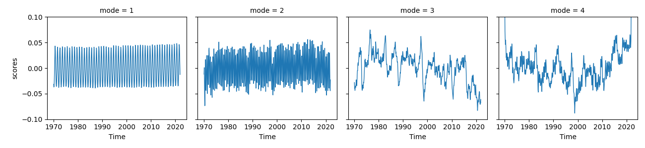
<xarray.plot.facetgrid.FacetGrid object at 0x7ffac67f2210>
And indeed the annual cycle is completed incorporated into the first mode, while the second mode shows a semi-annual cycle (mode 3 in standard EOF).
However, mode three and four look unusual. While showing some similarity to
ENSO (e.g. in mode 3 peaks in 1982, 1998 and 2016), they exhibit a “running away”
behaviour towards the boundaries of the time series.
This a common issue in complex EOF analysis which is based on the Hilbert transform (a convolution)
that suffers from the absence of information at the time series boundaries. One way to mitigate this
is to artificially extend the time series also known as padding. In xeofs, you can enable
such a padding by setting the padding parameter to "exp" which will extent the boundaries by an exponential
decaying function. The decay_factor parameter controls the decay rate of the exponential function measured in
multiples of the time series length. Let’s see how the decay parameter impacts the results:
model_ext = xe.models.ComplexEOF(padding="exp", decay_factor=0.01, **kwargs)
model_ext.fit(sst, dim="time")
scores_ext = model_ext.scores().sel(mode=slice(1, 4))

scores_ext.real.plot.line(x="time", col="mode", lw=1, ylim=(-0.1, 0.1))
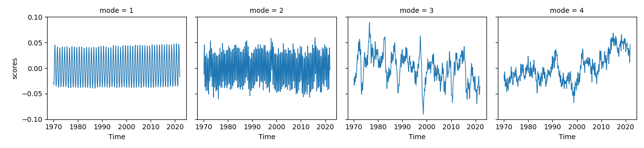
<xarray.plot.facetgrid.FacetGrid object at 0x7ffac75c1390>
And indeed, padding the time series effectively reduced the artifacts at the boundaries. Lastly, we examine the complex component amplitudes and phases.
comp_amps = model.components_amplitude()
comp_amps.plot(col="mode", vmin=0, vmax=0.025)
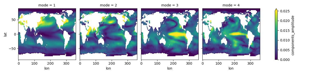
<xarray.plot.facetgrid.FacetGrid object at 0x7ffac63c67d0>
The component phases of the first mode clearly show the seasonal cycle as the northern and southern hemisphere are phase shifted by 180 degrees (white and black). Note the blueish regions in the central East Pacific and Indian Ocean which indicate a phase shift of 90 degrees compared to the main annual cycle. This is in agreement with mode 3 of the standard EOF analysis.
comp_phases = model.components_phase()
comp_phases.plot(col="mode", cmap="twilight")
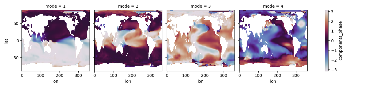
<xarray.plot.facetgrid.FacetGrid object at 0x7ffac7aee7d0>
Total running time of the script: (0 minutes 3.119 seconds)