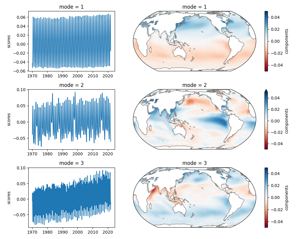
EOF analysis (S-mode)

EOF analysis in S-mode maximises the temporal variance.

# Load packages and data:
import xarray as xr
import matplotlib.pyplot as plt
from matplotlib.gridspec import GridSpec
from cartopy.crs import EqualEarth, PlateCarree

from xeofs.models import EOF

sst = xr.tutorial.open_dataset("ersstv5")["sst"]

Perform the actual analysis

model = EOF(n_modes=5, use_coslat=True)
model.fit(sst, dim="time")
expvar = model.explained_variance()
expvar_ratio = model.explained_variance_ratio()
components = model.components()
scores = model.scores()

Explained variance fraction

print("Explained variance: ", expvar.round(0).values)
print("Relative: ", (expvar_ratio * 100).round(1).values)

Explained variance:  [24398.  1066.   676.   407.   303.]
Relative:  [85.5  3.7  2.4  1.4  1.1]

Create figure showing the first two modes

proj = EqualEarth(central_longitude=180)
kwargs = {"cmap": "RdBu", "vmin": -0.05, "vmax": 0.05, "transform": PlateCarree()}

fig = plt.figure(figsize=(10, 8))
gs = GridSpec(3, 2, width_ratios=[1, 2])
ax0 = [fig.add_subplot(gs[i, 0]) for i in range(3)]
ax1 = [fig.add_subplot(gs[i, 1], projection=proj) for i in range(3)]

for i, (a0, a1) in enumerate(zip(ax0, ax1)):
    scores.sel(mode=i + 1).plot(ax=a0)
    a1.coastlines(color=".5")
    components.sel(mode=i + 1).plot(ax=a1, **kwargs)

    a0.set_xlabel("")

plt.tight_layout()
plt.savefig("eof-smode.jpg")