Complex EOF analysis

In this tutorial, we’ll walk through how to perform a Complex EOF analysis on the zonal and meridional wind components.

Let’s start by importing the necessary packages and loading the data:

import matplotlib.pyplot as plt
import xarray as xr

import xeofs as xe

xr.set_options(display_expand_attrs=False)

<xarray.core.options.set_options object at 0x7e85b3262450>

For this example, we’ll use the ERA-Interim tutorial dataset eraint_uvz:

uvz = xr.tutorial.open_dataset("eraint_uvz")
uvz

<xarray.Dataset>
Dimensions:    (longitude: 480, latitude: 241, level: 3, month: 2)
Coordinates:
  * longitude  (longitude) float32 -180.0 -179.2 -178.5 ... 177.8 178.5 179.2
  * latitude   (latitude) float32 90.0 89.25 88.5 87.75 ... -88.5 -89.25 -90.0
  * level      (level) int32 200 500 850
  * month      (month) int32 1 7
Data variables:
    z          (month, level, latitude, longitude) float64 ...
    u          (month, level, latitude, longitude) float64 ...
    v          (month, level, latitude, longitude) float64 ...
Attributes: (2)

xarray.Dataset

• Dimensions:
  • longitude: 480
  • latitude: 241
  • level: 3
  • month: 2
• Coordinates: (4)
  • longitude
    (longitude)
    float32
    -180.0 -179.2 ... 178.5 179.2

    units :

    degrees_east

    long_name :

    longitude

    array([-180.  , -179.25, -178.5 , ...,  177.75,  178.5 ,  179.25],
          dtype=float32)

  • latitude
    (latitude)
    float32
    90.0 89.25 88.5 ... -89.25 -90.0

    units :

    degrees_north

    long_name :

    latitude

    array([ 90.  ,  89.25,  88.5 , ..., -88.5 , -89.25, -90.  ], dtype=float32)

  • level
    (level)
    int32
    200 500 850

    units :

    millibars

    long_name :

    pressure_level

    array([200, 500, 850], dtype=int32)

  • month
    (month)
    int32
    1 7

    array([1, 7], dtype=int32)

• Data variables: (3)
  • z
    (month, level, latitude, longitude)
    float64
    ...

    number_of_significant_digits :

    5

    units :

    m**2 s**-2

    long_name :

    Geopotential

    standard_name :

    geopotential

    [694080 values with dtype=float64]

  • u
    (month, level, latitude, longitude)
    float64
    ...

    number_of_significant_digits :

    2

    units :

    m s**-1

    long_name :

    U component of wind

    standard_name :

    eastward_wind

    [694080 values with dtype=float64]

  • v
    (month, level, latitude, longitude)
    float64
    ...

    number_of_significant_digits :

    2

    units :

    m s**-1

    long_name :

    V component of wind

    standard_name :

    northward_wind

    [694080 values with dtype=float64]

• Indexes: (4)
  • longitude
    PandasIndex

    PandasIndex(Index([ -180.0, -179.25,  -178.5, -177.75,  -177.0, -176.25,  -175.5, -174.75,
            -174.0, -173.25,
           ...
             172.5,  173.25,   174.0,  174.75,   175.5,  176.25,   177.0,  177.75,
             178.5,  179.25],
          dtype='float32', name='longitude', length=480))

  • latitude
    PandasIndex

    PandasIndex(Index([  90.0,  89.25,   88.5,  87.75,   87.0,  86.25,   85.5,  84.75,   84.0,
            83.25,
           ...
           -83.25,  -84.0, -84.75,  -85.5, -86.25,  -87.0, -87.75,  -88.5, -89.25,
            -90.0],
          dtype='float32', name='latitude', length=241))

  • level
    PandasIndex

    PandasIndex(Index([200, 500, 850], dtype='int32', name='level'))

  • month
    PandasIndex

    PandasIndex(Index([1, 7], dtype='int32', name='month'))

• Attributes: (2)

  Conventions :

  CF-1.0

  Info :

  Monthly ERA-Interim data. Downloaded and edited by fabien.maussion@uibk.ac.at

This dataset contains the zonal, meridional, and vertical wind components at three different atmospheric levels. Note that the data only covers two months, so we have just two time steps (samples). While this isn’t enough for a robust EOF analysis, we’ll proceed for demonstration purposes. Now, let’s combine the zonal (u) and meridional (v) wind components into a complex-valued dataset:

Z = uvz["u"] + 1j * uvz["v"]

Next, we’ll initialize and fit the ComplexEOF model to our data. The xeofs package makes this easy by allowing us to specify the sample dimension (month), automatically performing the Complex EOF analysis across all three atmospheric levels. As a standard practice, we’ll also weigh each grid cell by the square root of the cosine of the latitude (use_coslat=True).

model = xe.single.ComplexEOF(n_modes=1, use_coslat=True, random_state=7)
model.fit(Z, dim="month")

/home/nrieger/miniconda3/envs/xeofs/lib/python3.11/site-packages/scipy/sparse/linalg/_eigen/_svds.py:483: UserWarning: The problem size 2 minus the constraints size 0 is too small relative to the block size 1. Using a dense eigensolver instead of LOBPCG iterations.No output of the history of the iterations.
  _, eigvec = lobpcg(XH_X, X, tol=tol ** 2, maxiter=maxiter,

<xeofs.single.eof.ComplexEOF object at 0x7e85b3299950>

Instead of just extracting the complex-valued components, we can also get the amplitude and phase of these components. Let’s start by looking at the amplitude of the first mode:

spatial_ampltiudes = model.components_amplitude()
spatial_phases = model.components_phase()

spatial_ampltiudes.sel(mode=1).plot(col="level")
plt.show()

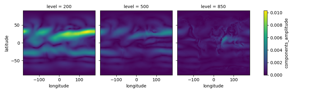
It looks like the first mode picks up a pattern resembling the location of the subtropical jet stream around ±30º latitude, particularly strong in the upper troposphere at 200 hPa and weaker toward the surface. We can also plot the phase of the first mode. To keep the plot clear, we’ll only show the phase where the amplitude is above a certain threshold (e.g., 0.004):

relevant_phases = spatial_phases.where(spatial_ampltiudes > 0.004)
relevant_phases.sel(mode=1).plot(col="level", cmap="twilight")
plt.show()